Ocean Temperature Data Exploring
Setup
Analysis and visualization was done using R and various packages. The following is the script used to generate 2 scatterplot graphs.
library(tidyverse)
library(lubridate)
library(ggplot2)
library(plotly)
options(repr.plot.width=10, repr.plot.height=6)
Reading and Wrangling Data
Temperature data [Dewees and NOAA Office of Marine and Aviation Operations, 2021] are found in the "data" folder, while coordinates (and the time recorded) are in the "data/nav" folder.
All of the temperature data was cleaned using a Python script, located in the data_cleaning folder. No packages were used, and can be used as long as a v3.9 Python is installed (anything above or below is untested) and the scripts are pointed to the right data sources.
data/temp_processed_summarized.csv: mean temp over mindata/nav/nav_processed.csv: mean GPS over mindata/nav_temp_joined_processed.csv: joined mean temp & GPS over min
The dates are all of type character, meaning extracting any use without it being a proper date type is hard. Therefore, time and date must be formatted.
format_datetime <- function(df) {
df_new <- df %>%
# https://www.neonscience.org/resources/learning-hub/tutorials/dc-time-series-subset-dplyr-r
mutate(date = as.Date(date, format = '%m/%d/%Y')) %>%
# https://www.tidyverse.org/blog/2021/03/clock-0-1-0/
mutate(datetime = as.POSIXct(date, "America/Vancouver")) %>%
mutate(datetime = datetime +hour(time)+ minute(time))
return(df_new)
}
The following are all of the functions needed to clean up 1 temperature file. However, we have quite a few files, and trying to clean and instantiate each by hand is cumbersome. Therefore, we will iterate through all of the files and summarize.
Attention
Please keep in mind that the following code blocks will take pretty long to run.
clean_SBE45_data <- function(x) {
read <- read_delim(x, delim = ",",
col_names = c("date",
"time",
"int_temp",
"conductivity",
"salinity",
"sound_vel",
"ext_temp"),
col_types = cols(
date = col_character(),
time = col_time(format = ""),
int_temp = col_double(),
conductivity = col_double(),
salinity = col_double(),
sound_vel = col_double(),
ext_temp = col_double()
)) %>%
select(date, time, ext_temp)
return(read)
}
clean_STT_TSG_data <- function(x) {
read <- read_delim(x, delim = ",",
col_names = c("date",
"time",
"type",
"diff",
"ext_temp",
"int_temp",
"extra")
) %>%
select(date, time)
return(read)
}
clean_temp_data <- function(x) {
# https://stackoverflow.com/questions/10128617/test-if-characters-are-in-a-string
if(grepl("SBE45-TSG-MSG", x, fixed = TRUE)) {
return(clean_SBE45_data(x))
} else {
return(clean_STT_TSG_data(x))
}
}
This is the data before it is summarized by the minute.
# https://stackoverflow.com/questions/11433432/how-to-import-multiple-csv-files-at-once
all_temperature_loaded <- list.files(path = "data/",
pattern = "*.Raw",
full.names = T) %>%
map_df(~clean_temp_data(.))
head(all_temperature_loaded)
summary(all_temperature_loaded)
| date | time | ext_temp |
|---|---|---|
| 06/13/2021 | 19:42:03 | 19.5731 |
| 06/13/2021 | 19:42:04 | 19.5240 |
| 06/13/2021 | 19:42:05 | 19.4795 |
| 06/13/2021 | 19:42:06 | 19.4724 |
| 06/13/2021 | 19:42:07 | 19.4734 |
| 06/13/2021 | 19:42:08 | 19.4718 |
date time ext_temp
Length:7267565 Length:7267565 Min. : 0
Class :character Class1:hms 1st Qu.:13
Mode :character Class2:difftime Median :15
Mode :numeric Mean :15
3rd Qu.:17
Max. :24
NA's :3687228
all_temperature_cleaned <- all_temperature_loaded %>%
filter(!is.na(ext_temp)) %>%
filter(ext_temp > 2) %>%
format_datetime()
all_temperature <- group_by(all_temperature_cleaned, datetime) %>%
summarize(mean_ext = mean(ext_temp, na.rm = TRUE))
write_csv(all_temperature, "data/temp_processed_summarized.csv")
head(all_temperature)
summary(all_temperature)
| datetime | mean_ext |
|---|---|
| 2021-06-12 17:00:20 | 19.05565 |
| 2021-06-12 17:00:21 | 18.62864 |
| 2021-06-12 17:00:22 | 19.00354 |
| 2021-06-12 17:00:23 | 19.09503 |
| 2021-06-12 17:00:24 | 19.17977 |
| 2021-06-12 17:00:25 | 19.10705 |
datetime mean_ext
Min. :2021-06-12 17:00:20 Min. : 9.618
1st Qu.:2021-06-23 17:00:13 1st Qu.:13.096
Median :2021-07-04 17:00:06 Median :14.771
Mean :2021-07-04 07:00:13 Mean :15.165
3rd Qu.:2021-07-15 11:00:20 3rd Qu.:16.586
Max. :2021-07-25 17:01:16 Max. :24.086
All of the navigation files will also be cleaned up and summarized in similar manner to the temperature files.
clean_nav_data <- function(x) {
read <- read_csv(x,
col_names = c(
"date",
"time",
"type",
"time_num",
"lat",
"lat_NS",
"long",
"long_WE",
"gps_quality",
"num_sat_view",
"hort_dil",
"ant_alt",
"ant_alt_unit",
"geoidal",
"geoidal_unit",
"age_diff",
"diff_station"
)
) %>%
select(date, time, lat, long)
return(read)
}
Below is the raw ocean navigation data.
all_nav_loaded <- list.files(path = "data/nav/",
pattern = "*.Raw",
full.names = T) %>%
map_df(~clean_nav_data(.)) %>%
format_datetime()
summary(all_nav_loaded)
date time lat long
Min. :2021-06-13 Length:3722834 Min. :3132 Min. :11709
1st Qu.:2021-06-24 Class1:hms 1st Qu.:3341 1st Qu.:12045
Median :2021-07-05 Class2:difftime Median :3750 Median :12310
Mean :2021-07-04 Mode :numeric Mean :3922 Mean :12285
3rd Qu.:2021-07-15 3rd Qu.:4537 3rd Qu.:12456
Max. :2021-07-26 Max. :5224 Max. :13053
datetime
Min. :2021-06-12 17:00:16
1st Qu.:2021-06-23 17:00:37
Median :2021-07-04 17:00:24
Mean :2021-07-04 09:56:25
3rd Qu.:2021-07-14 17:01:16
Max. :2021-07-25 17:01:16
Since the latitude and longitude are in the degree minutes format, they must be converted.
all_nav <- all_nav_loaded %>%
group_by(datetime) %>%
summarize(mean_lat = mean(lat), mean_long = mean(long)) %>%
mutate(mean_lat = mean_lat/100, mean_long = mean_long/100) %>%
mutate(deg_lat_int = trunc(mean_lat, 0),
deg_long_int = trunc(mean_long, 0)) %>%
mutate(deg_lat_dec = round((mean_lat - deg_lat_int) * 10000),
deg_long_dec = round((mean_long - deg_long_int) * 10000)) %>%
mutate(mean_deg_lat = deg_lat_int + deg_lat_dec/(60 * 100),
mean_deg_long = deg_long_int + deg_long_dec / (60 * 100)) %>%
select(-deg_lat_int, -deg_long_int, -deg_lat_dec, -deg_long_dec, -mean_lat, -mean_long)
write_csv(all_nav, "data/nav/nav_processed.csv")
head(all_nav)
summary(all_nav)
| datetime | mean_deg_lat | mean_deg_long |
|---|---|---|
| 2021-06-12 17:00:16 | 32.69633 | 117.1570 |
| 2021-06-12 17:00:17 | 32.69650 | 117.1568 |
| 2021-06-12 17:00:18 | 32.69683 | 117.1563 |
| 2021-06-12 17:00:19 | 32.69283 | 117.1755 |
| 2021-06-12 17:00:20 | 32.67333 | 117.2213 |
| 2021-06-12 17:00:21 | 32.66167 | 117.2897 |
datetime mean_deg_lat mean_deg_long
Min. :2021-06-12 17:00:16 Min. :31.54 Min. :117.2
1st Qu.:2021-06-23 17:00:10 1st Qu.:33.71 1st Qu.:120.6
Median :2021-07-04 17:00:04 Median :37.83 Median :123.3
Mean :2021-07-04 06:25:58 Mean :39.40 Mean :123.1
3rd Qu.:2021-07-14 17:01:21 3rd Qu.:45.25 3rd Qu.:125.0
Max. :2021-07-25 17:01:16 Max. :52.64 Max. :130.8
Since we have the date and time (by the minute) of both the temperature and it’s coordinates, we can match the two columns.
joined_temp_nav <- inner_join(all_temperature,
all_nav,
by = c("datetime" = "datetime"))
write_csv(joined_temp_nav, "data/nav_temp_joined_processed.csv")
head(joined_temp_nav)
summary(joined_temp_nav)
| datetime | mean_ext | mean_deg_lat | mean_deg_long |
|---|---|---|---|
| 2021-06-12 17:00:20 | 19.05565 | 32.67333 | 117.2213 |
| 2021-06-12 17:00:21 | 18.62864 | 32.66167 | 117.2897 |
| 2021-06-12 17:00:22 | 19.00354 | 32.65833 | 117.3313 |
| 2021-06-12 17:00:23 | 19.09503 | 32.65250 | 117.3740 |
| 2021-06-12 17:00:24 | 19.17977 | 32.65217 | 117.3750 |
| 2021-06-12 17:00:25 | 19.10705 | 32.65183 | 117.3758 |
datetime mean_ext mean_deg_lat mean_deg_long
Min. :2021-06-12 17:00:20 Min. : 9.618 Min. :31.54 Min. :117.2
1st Qu.:2021-06-23 17:00:13 1st Qu.:13.096 1st Qu.:33.74 1st Qu.:120.6
Median :2021-07-04 17:00:06 Median :14.771 Median :37.83 Median :123.4
Mean :2021-07-04 07:00:13 Mean :15.165 Mean :39.41 Mean :123.1
3rd Qu.:2021-07-15 11:00:20 3rd Qu.:16.586 3rd Qu.:45.25 3rd Qu.:125.0
Max. :2021-07-25 17:01:16 Max. :24.086 Max. :52.64 Max. :130.8
Visualizing the Data
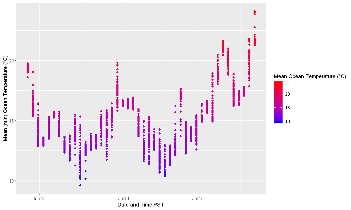
Time and mean temperature plotted on a scatterplot to see temperature changes over time. Notice that since the ship moves in 1 way vs time, the shape of the 2D scatterplot and the 3D plot is very similar.
time_plot <- ggplot(all_temperature, aes(x = datetime,
y = mean_ext,
colour = mean_ext)) +
geom_point() +
scale_colour_gradient(low = "blue", high = "red") +
labs(x = "Date and Time PST",
y = "Mean (min) Ocean Temperature (°C)",
colour = "Mean Ocean Temperature (°C)")
time_plot
p<- plot_ly(joined_temp_nav,
x = ~mean_deg_lat,
y = ~mean_deg_long,
z = ~mean_ext,
color = ~mean_ext
) %>%
add_markers(size = 0.7) %>%
colorbar(title = "Mean Ocean Temp (°C)")%>%
layout(title = "Mean Ocean Temperature and Coordinates",
scene = list(
xaxis = list(title = "Mean Latitude (°)"),
yaxis = list(title = "Mean Longitude (°)"),
zaxis = list(title = "Mean Ocean Temp (°C)")
)
)
embed_notebook(p)